Autoregressive Integrated Moving Average (ARIMA) is a popular time series forecasting model. It is used in forecasting time series variable such as price, sales, production, demand etc.

1. Basics of ARIMA model

As the name suggests, this model involves three parts: Autoregressive part, Integrated and Moving Average part. Let us explore these parts one by one.

A) Autoregressive part

Autoregressive part refers to relationship between the variable (that we are trying to forecast) with its own lagged values. The order of AR term is denoted by p. If p=2, that means the variable depends upon past two lagged values. In case of seasonal ARIMA model, the seasonal AR part is denoted by the notation P.

• If P is let us say, 1, then that means the time series variable depends on the value for the same period during the last season. For example, if it is monthly data, then the value observed during March this year is dependent on value observed during last year March.
• While the non-seasonal AR order 2 indicates the value observed during March this year is dependent on value observed during February and January of this year.
• What will be the meaning of AR seasonal order P = 3 in case of monthly data? That means, if the present month is March, 2018 then time series value for this month is dependent on values during March 2017, March 2016 and March 2015.

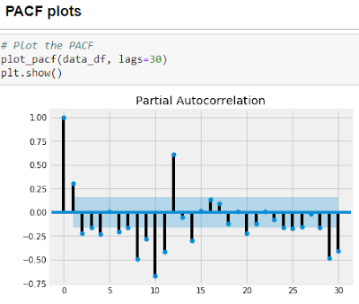
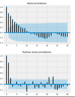
The order of AR part can be inferred from the Partial Auto-Correlation Function (PACF) plot.

B) Integrated part

Integrated part refers to order of differencing. Non-seasonal differencing order is denoted by d and seasonal differencing order by D. Integrated part is essential when the series is non-stationary.

C) Moving Average part

In ARIMA model, Moving Average order indicates the dependence of present value of the time series variable on the lagged error terms. The non-seasonal MA order is denoted by q while the seasonal MA order is denoted by Q.

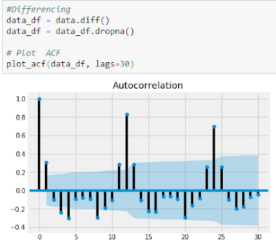
The order of MA part can be inferred from the Auto-Correlation Function (ACF) plot.

The following picture depicts a SARIMA model of the order (p,d,q)(P,D,Q)_m (Fore more on this).

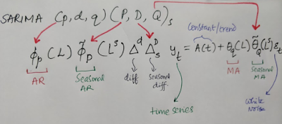
SARIMA (p,d,q)(P,D,Q)_m

where L is the backshift operator.

2. Example in Python

Using the famous Airline Passengers dataset, let us build the ARIMA model.

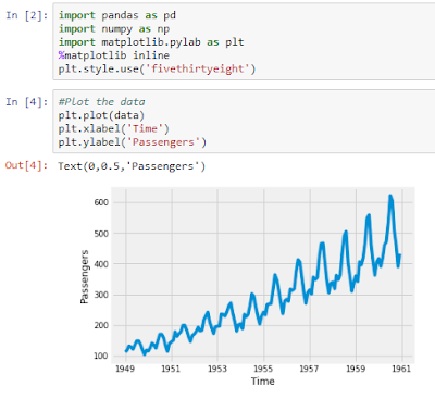
a) Auto-Correlation Function (ACF) plot

Let us plot ACF

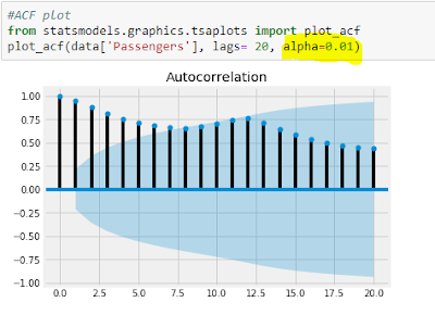
ACF plot with 99% Confidence Intervals

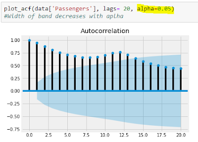
ACF plot with 95% Confidence Intervals

As you can see from these ACF plots, width of the confidence interval band decreases with increase in alpha value. These ACF plots and also the earlier line graph reveal that time series requires differencing (Further use ADF or KPSS tests)If you want to get ACF values, then use the following code.

b) Partial Auto-Correlation Function (PACF) plot

Now let us plot PACF

c) Seasonal differencing

d) Fitting the model

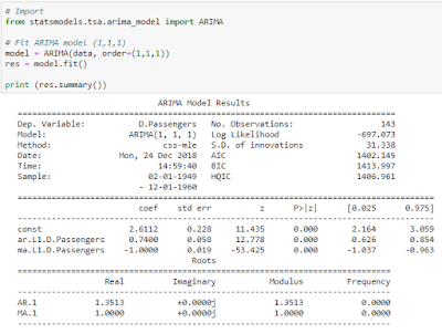
i) ARIMA

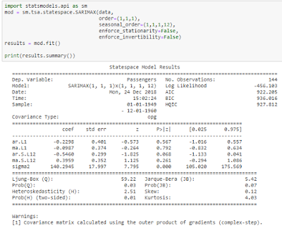
ii) SARIMA

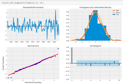
e) Diagnostic Plots

We want the residuals to be white noise process.

f) Forecasting

In case of ARIMA model, we can use the following code:

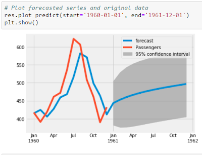
To get the confidence intervals and standard error, we can use the following code:

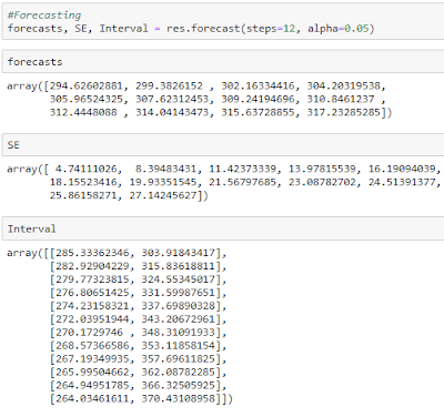
In case of SARIMA model, we need to use the following code:

a) Forecast and confidence intervals

We can get the summary of the forecasts using summary_frame() function.

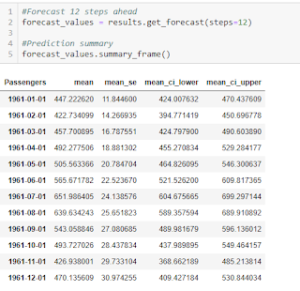
Or alternatively, we can get the prediction and confidence intervals for the predictions as shown below.

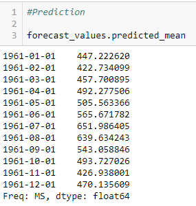
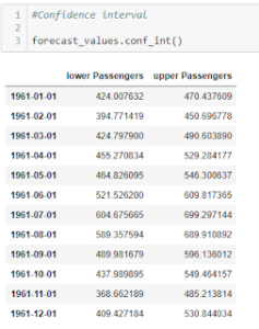
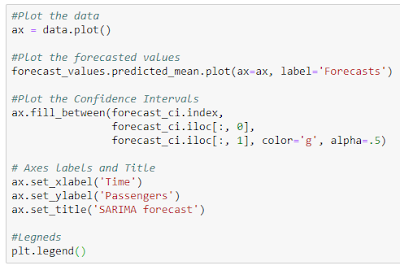
b) Plot the forecasted values and confidence intervals

For this, I have used the code from this blog-post, and modified it accordingly.

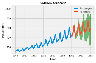
Further, we can use dynamic forecasting which uses the forecasted time series variable value instead of true time series value for prediction. But generally it does not perform as good as the normal static method.

Points to consider:

• Generally total order of differencing (d+D) should be not more than two.
• Even though we derive p and P values from PACF plots and q and Q values from ACF plots, we have to overfit, check residues, check performance. Model building is an art which requires us to consider various points before shortlisting the models.
• AIC should be used to compare the models with the same order of differencing (link).

Summary

In this post, we have explored

• the basics of ARIMA/SARIMA models and
• how to forecast using these models in Python

References:

• https://otexts.org/fpp2/seasonal-arima.html
• https://www.statsmodels.org/dev/generated/statsmodels.tsa.statespace.sarimax.SARIMAXResults.get_prediction.html
• http://www.statsmodels.org/dev/examples/notebooks/generated/statespace_sarimax_stata.html
• https://www.digitalocean.com/community/tutorials/a-guide-to-time-series-forecasting-with-arima-in-python-3
• https://otexts.org/fpp2/residuals.html
• https://otexts.org/fpp2/prediction-intervals.html#prediction-intervals
• http://barnesanalytics.com/basics-of-arima-models-with-statsmodels-in-python
• http://barnesanalytics.com/sarima-models-using-statsmodels-in-python