Understanding Naive Bayes using simple examples
Thomas Bayes was an English statistician. As Stigler states, Thomas Bayes was born in 1701, with a probability value of 0.8! (link). Bayes’ theorem has a useful application in machine learning. His papers were published by his friend, after his death. It is also said that his friend has used the theorem to prove existence of God.
Bayes’ Theorem
Using Bayes’ theorem, we can solve ‘inverse probability’ problems. Though the term ‘inverse probability’ is not used nowadays, I used it because it helps you to understand the concept which I am going to explain now.
Imagine you know the probability of an email being a spam email. You also know the probability of occurrence of word “discount” given the email is spam. And, you also know the probability of occurrence of word “discount” in any email. Can you now find out the probability of a given email being spam if it contains the word “discount”? It is like inverse probability, isn’t it?
Bayes’ theorem helps to solve this problem. Now let us go through the question once again, step by step, with explanation.
- “you know the probability of an email being spam email”
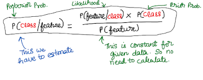
This is called prior probability which I showed using an arrow in the following picture (equation 1). In equation 1, class refers to spam email. Feature refers to occurrence of word “discount”. Now let us move ahead to the next sentence of the problem.
- “You also know the probability of occurrence of word “discount” given the email is spam”
This is a conditional probability called as the likelihood. Now the next sentence.
- “you also know the probability of occurrence of word “discount”in any email”
This refers to the evidence or normalizing constant . The denominator part of the equation 1 is P(feature). We don’t calculate the value of this denominator in naive bayes estimation. We will discuss the reason later. Now the last sentence of the problem.
- “Can you now find out the probability of a given email being spam if it contains the word “discount”?
This is the left hand side of the equation 1. Using the following equation, we can calculate the probability of a given email being spam when an email contains the word “discount”.

Equation 1 – Bayes’ theorem
In reality, we need more than one feature to fit a classification model. In the following example, I have used three features (or three independent variables: x1, x2 and x3). The three features are the occurrence of words “discount”, “money” and “hurry”.
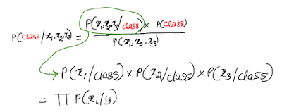
We can modify the above equation to incorporate these three independent variables. To simplify the first term in the numerator of equation 2 (also called the likelihood), we assume conditional independence of features given the class. And because of this naive assumption, this classification techniques gets its name – naive bayes. What does this assumption mean?
This means, given the class of the email (let us say the email is a spam), then probability of occurrences of words “discount”, “money”, “hurry” are independent. Though it may not hold good in reality, but this assumption helps to simplify the equation 2. Since the features are independent, we can now multiply the conditional probability values of each of these three features given the class and sum these values to get the likelihood value as shown below.

Equation 2 – Assumption of conditional independence of features helps to simplify likelihood term of the numerator
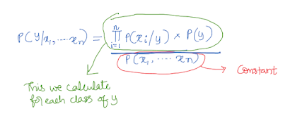
Now instead of class let us use “y” and rewrite the equation 2 in the following format (equation 3). This is the final equation we use to build the naive bayes classifier. If there are three classes, then we have to calculate the probability values for each of the three classes using the given feature values. But we don’t have to calculate the denominator, why? Because even if you calculate the denominator value it will be the same for the given data. Confused? Okay, let me give you an example.
Let us say there are two classes. For the first class, lets say numerator value is 0.4 and for the second class it is 0.6. And the denominator value is 0.9 for both these classes. Then we can divide 0.4 by 0.9 (=0.44) and divide 0.6 by 0.9 (=0.67) and find out which class has higher probability (0.67 > 0.44). Instead of dividing by the same denominator value, we can directly compare the numerator (0.6 > 0.4) and find out which has higher value in the numerator (naturally higher the numerator value, higher will be the probability value given a constant denominator) and predict the class accordingly.

Equation 3 – Naive Bayes classification rule
Gaussian Naive Bayes
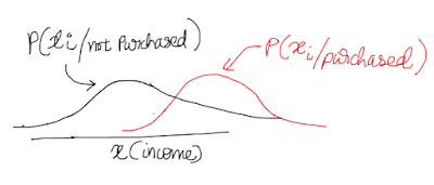
Here the assumption is that the feature values (continuous variable like income) are normally distributed in each class. Look at the following picture where there are two classes (not purchased and purchased). In each of these two classes, the independent variable or the feature (income) is assumed to be normally distributed. Using this assumption, we calculate the likelihood term of the bayes’ equation.

Example (naive bayes using python)
#Import

from sklearn import datasets
iris = datasets.load_iris()
from sklearn.naive_bayes import GaussianNB
from sklearn.model_selection import train_test_split
from sklearn.metrics import accuracy_score

#Data
X=iris.data
y=iris.target

#Splitting into test and train
x_train, x_test, y_train, y_test = train_test_split(X, y, test_size=0.2, random_state=0)

#Fit Naive Bayes
gnb = GaussianNB()
gnb.fit(x_train, y_train)
Output: GaussianNB(priors=None)
#Prediction and accuracy
y_pred = gnb.predict(x_test)
accuracy_test = accuracy_score(y_test, y_pred)

#Print accuracy
print ("Test Accuracy: %0.2f" % (accuracy_test))
Output: Test Accuracy: 0.97
In this blogpost, we have understood the Bayes’ theorem and its application with python for solving classification tasks.

