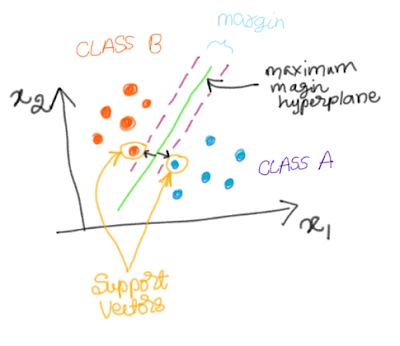
Suppose there are two independent variables (features): x1 and x2. And there are two classes Class A and Class B. The following graphic shows the scatter diagram.
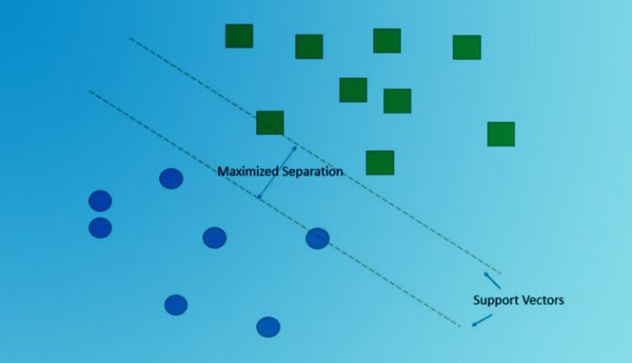
If want to partition these two classes using a line (or hyperplane), the green hyperplane will seperate the two classes with maximum margin between the two classes. The data points which decide the margin are called support vectors. In other words, these are the points that lie closest to the decision surface (link).

Support Vectors
To understand why there points are called support vectors, read this excellent blog. According this blogpost, since these two points ‘support’ the hyperplane to be in ‘equilibrium’ by exerting torque (mechanical analogy), these data points are called as the support vectors.
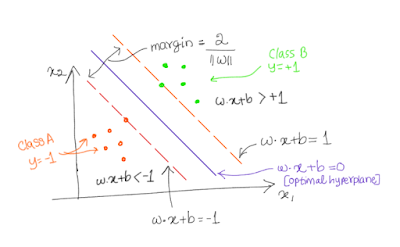
In the following figure, there are two classes: positive classes (where y=+1) and negative classes (where y= -1). We need to find out a hyperplane which maximizes the margin. Since there are two features (x1 and x2) which means p=2. And we need to find out a hyperplance of the dimension p-1. In our case, dimension of hyperplane is 2-1=1.

Equations
Advantages
- Performs well in higher dimensional spaces (where p is higher relative to n)
- Memory efficient
Disadvantage
- Probability estimates need to be derived indirectly
- Problem of overfitting
Example
The data used for demonstrating the logistic regression is from the Titanic dataset. For simplicity I have used only three features (Age, fare and pclass).
And I have performed 5-fold cross-validation (cv=5) after dividing the data into training (80%) and testing (20%) datasets. I have calculated accuracy using both cv and also on test dataset.
1) SVM with linear kernel
We will see how to fit SVM with linear kernel and how to perform CV.
#Ravel
y=y.values.ravel()

#import
from sklearn import svm
from sklearn.model_selection import train_test_split

#Splitting
x_train, x_test, y_train, y_test = train_test_split(X, y, test_size=0.2, random_state=0)

#SVC with Linear kernel
svc = svm.SVC(kernel='linear')

#Fit
svc.fit(x_train, y_train)
    SVC(C=1.0, cache_size=200, class_weight=None, coef0=0.0,
  decision_function_shape='ovr', degree=3, gamma='auto', kernel='linear',
  max_iter=-1, probability=False, random_state=None, shrinking=True,
  tol=0.001, verbose=False)
from sklearn.model_selection import cross_val_score
from sklearn.metrics import accuracy_score

#CV scores, 5 fold CV
scores = cross_val_score(svc, x_train, y_train, cv=5)

#Prediction and accuracy
y_pred = svc.predict(x_test)
accuracy_test = accuracy_score(y_test, y_pred)

#Print the summary
print("Accuracy: %0.2f (+/- %0.2f)" % (scores.mean(), scores.std() * 2))
print ("Test Accuracy: %0.2f" % (accuracy_test))
Accuracy: 0.69 (+/- 0.03)
Test Accuracy: 0.70
2) SVM with polynomial kernel
#SVC with polynomial kernel
svc = svm.SVC(kernel='poly', degree=2)

#Fit
svc.fit(x_train, y_train)
SVC(C=1.0, cache_size=200, class_weight=None, coef0=0.0, decision_function_shape=’ovr’, degree=2, gamma=’auto’, kernel=’poly’, max_iter=-1, probability=False, random_state=None, shrinking=True, tol=0.001, verbose=False)
3) SVM with rbf kernel
#SVC with rbf kernel
svc = svm.SVC(kernel='rbf')

#Fit
svc.fit(x_train, y_train)
SVC(C=1.0, cache_size=200, class_weight=None, coef0=0.0, decision_function_shape=’ovr’, degree=3, gamma=’auto’, kernel=’rbf’, max_iter=-1, probability=False, random_state=None, shrinking=True, tol=0.001, verbose=False)
4) LinearSVC with linear kernel
#Linear SVC with Linear Kernel
from sklearn.svm import LinearSVC

clf = LinearSVC()
clf.fit(X, y)
LinearSVC(C=1.0, class_weight=None, dual=True, fit_intercept=True, intercept_scaling=1, loss=’squared_hinge’, max_iter=1000, multi_class=’ovr’, penalty=’l2′, random_state=None, tol=0.0001, verbose=0)
In this case, squared hinge loss function (as against hinge loss function) and l2 penalty are the major changes compared to the earlier three methods. This method is useful for when sample size is larger.
For more on Linear SVC, you may refer this manual.
Hyperparameters
Let us learn about the important hyperparameters of SVM.
- C
- It is the cost of misclassification. Smaller C means lower cost of misclassification, that means wider margin. Larger value of C means higher chance of overfitting because of smaller margin.
- Kernel
- ‘linear’, ‘poly’, ‘rbf’ are the major kernels used in SVM.
- Class weight
- The ‘balanced’ mode by automatically adjusting the class weights to inverse of frequencies in each class. This is useful while handling class imbalance in dataset.
- Fit Intercept
- By default, intercept is added to the logistic regression model.
- decision_function_shape
- The one-vs-rest (‘ovr’) is the default option. The ‘ovo’ option corresponds to one-vs-one.
- gamma
- The gamma parameter corresponds to inverse of radius of influence of support vector data points (source). That means if gamma is too large, that means influence of support vectors is limited only to themselves which lead to overfitting.In future, ‘scale’ will be used as the default option.
- degree
- Only when the kernel used is ‘poly’, 3 is the default option.
Tuning Hyperparameters
Let us explore how to tune important hyperparemeters in SVM. We can use either grid search or randomized search methods.
In this example, I grid search for best hyperparameters.
#import GridseachCV
from sklearn.model_selection import GridSearchCV
from sklearn import svm

#Instantiate
svc = svm.SVC()

#Grid
param_grid = [
    {'C': [1, 10, 100, 1000], 'kernel': ['linear']},
  {'C': [1, 10, 100, 1000], 'gamma': [0.001, 0.0001], 'kernel': ['rbf']}, ]

#Gridsearch
gridsearch = GridSearchCV(svc, param_grid)
gridsearch.fit(x_train, y_train);

#Get best hyperparameters
gridsearch.best_params_
{‘C’: 100, ‘gamma’: 0.001, ,’kernel’: ‘rbf’}
Additionally, we can also use randomized search for finding the best parameters. Advantages of randomized search is that it is faster and also we can search the hyperparameters such as C over distribution of values.
Summary
In this post, we have explored the basic concepts regarding SVM, advantages, disadvantages and example with Python. We have also learnt how to tune the hyperparameters to obtain better performance.
References
https://scikit-learn.org/stable/modules/svm.html
https://medium.com/@aneesha/svm-parameter-tuning-in-scikit-learn-using-gridsearchcv-2413c02125a0
https://scikit-learn.org/stable/modules/generated/sklearn.svm.SVC.html#sklearn.svm.SVC

