The concept of degrees of freedom is essential in statistical analysis, and it is commonly used in various statistical tests. In this blog post, we will explore A) Without any restriction B) With a restriction C) Degrees of freedom in contingency tables D) Bessel’s correction with examples. This will help you to understand degrees of freedom in a simple and effective way.

A) Without any restriction

Suppose we have three boxes, and we can fill them with any values of our choice. In this case, we have three degrees of freedom (df=n).

B) With a restriction

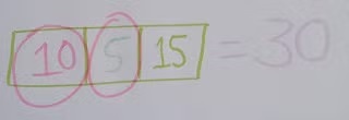
If we impose a restriction, such as the sum of the values in the boxes should be 30, then we lose one degree of freedom. For instance, if we fill the first box with 10, we can choose the value for only two boxes, and hence the degrees of freedom become 2 (df=n-1).

Let us imagine you filled the first cell with 10. Now you are left with 2 boxes.

And you fill the second box with 5. Now as the sum should be 30, you have to fill the third cell with 15.

Hence, even though there were three cells, you were free to choose values for 2 cells. Hence, in this case, the degrees of freedom is 2. In other words, df=(n-1) here.

C) Degrees of freedom in contingency tables

In contingency tables, the degrees of freedom are calculated as (row-1)*(column-1). For example, in a 2×2 contingency table, we have one degree of freedom, in a 2×3 table, we have two degrees of freedom, and in a 3×3 table, we have four degrees of freedom.

1) Degrees of freedom in 2×2 contingency table

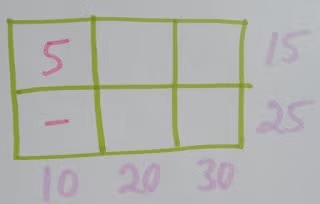
Suppose you are given with a 2×2 table with row and column totals. You have to fill the values in four cells, but the row and column totals should be equal to the given values.

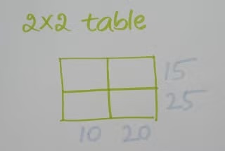
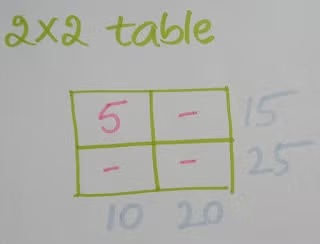
And you start with the first cell by filling it with 5. You now have no freedom to fill other values. Hence the degree of freedom is 1. Here, (row-1)*(column-1) = (2-1)*(2-1)= 1.

2) Degrees of freedom in 2×3 contingency table

Let us extend the same example to 2×3 table.

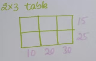
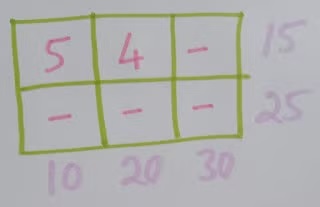
Imagine you filled the first cell with 5.

You are free to fill one more cell. And you fill it with 4. That’s all. No more freedom. Hence, degrees of freedom is 2. Here, (row-1)*(column-1) = (2-1)*(3-1)= 2.

3) Degrees of freedom in 3×3 contingency table

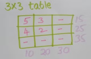
Here, as you can see, you are free to fill 4 cells. Hence, degrees of freedom is 4. Here, (row-1)*(column-1) = (3-1)*(3-1)= 4.

D) Bessel’s correction

When estimating the sample variance, we use (n-1) instead of n in the denominator. This is because we have already used one degree of freedom in estimating the sample mean, and hence we are left with (n-1) degrees of freedom to estimate the sample variance.

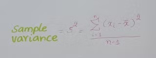
As you can see in the denominator, (n-1) is used instead of n.

What could be the reason? When we are estimating sample variance (or the sample standard deviation), we also need sample mean. For estimating the sample mean, we have already used one of the degrees of freedom.

Hence, now we are left with (n-1) degrees of freedom for estimating the sample variance (or the sample standard deviation). This is called Bessel’s correction.

Summary

In summary, degrees of freedom are the number of independent values that can be varied in a statistical analysis. The formula for calculating degrees of freedom is (sample size) – (number of parameters to be estimated).