Let’s explore the Central Limit Theorem (CLT) with an example of rolling two dice multiple times (let’s say 30 times). We will calculate the mean of the two dice values and plot its distribution to understand the CLT intuitively.

Round 1:

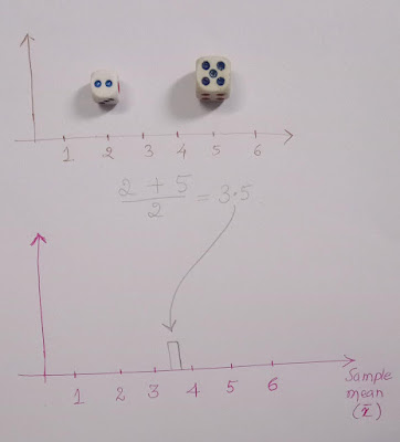
We roll the dice and get 2 and 5. The sample mean of 2 and 5 is 3.5.

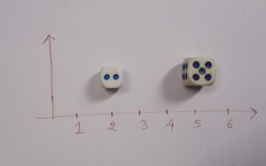
We plot this mean (3.5) in a plot.

Round 2:

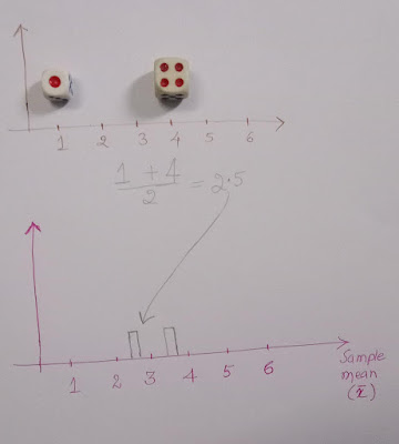
We roll the dice again and get 1 and 4. The mean of 1 and 4 is 2.5. We mark this mean on our plot.

Round 3:

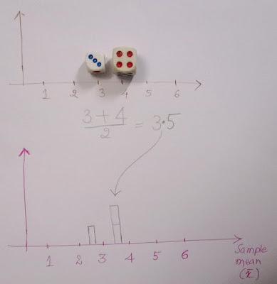
We roll the dice once more and get 3 and 4. The mean of 3 and 4 is 3.5. We mark this mean on our plot.

Round n:

We continue this process for many rounds, let’s say 30 or 100 rounds, and mark all the sample means on our plot. This plot is called the sampling distribution of the mean. As we increase the number of rounds, the sampling distribution of the mean approaches a normal distribution.

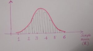
Even though the original data follows a uniform distribution (each value from 1 to 6 has an equal chance of occurring), the sampling distribution of the mean follows a normal distribution.

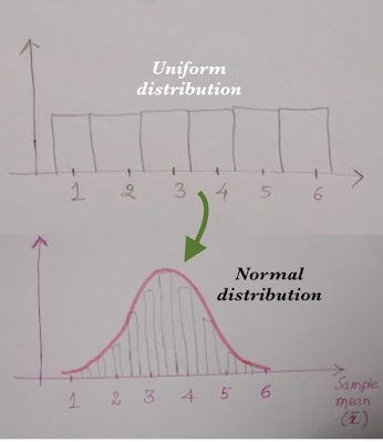
This is the essence of the Central Limit Theorem, which says that for sufficiently large random samples, the sample means will be normally distributed regardless of the distribution of the data.

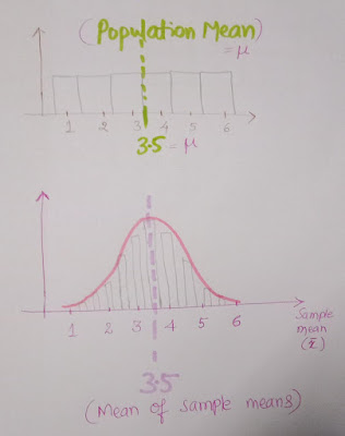
Moreover, the mean of sample means is equal to the population mean, and the standard deviation of sample means is the population standard deviation divided by the square root of the sample size.

Conclusion

In conclusion, this example helps us understand the Central Limit Theorem intuitively by demonstrating how the sampling distribution of the mean approaches normal distribution for sufficiently large random samples, regardless of the underlying distribution of the data.