Decision Tree models are simple and easy to interpret.
In this post, let us explore
- What are decision trees
- When to use decision trees
- Advantages
- Disadvantages
- Examples with code (Python)
1. What are decision trees?
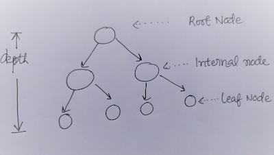
Decision trees are a tree like non-parametric supervised learning method.
Components of decision tree:

Root Node: It has no parent nodes.
Internal nodes: Have both parent and child nodes.
Leaf nodes: Don’t have child nodes. Also called terminal nodes.
Depth: In the above example, depth is two.
2. When to use decision trees?
Decision trees can be used for both classification and regression tasks. Decision trees handle both numerical and categorical data. Decision trees are non-linear models.
Decision trees are also used by default in
- Random Forests
- BaggingClassifier
- AdaBoostClassifier
- GradientBoostingClassifier
3. Advantages of Decision Trees
- Simple and can be visualized in the tree form
- No assumption about the distribution of data (non parametric method)
- Not much of data preprocessing is needed
- No need for data normalization and to create dummy variables
- Handles outliers well
- White box model: so easier to interpret the results
4. Disadvantages and steps to overcome
- Overfitting: decision trees can learn ‘too much’ from training data and may not perform well on testing data
- setting maximum depth of tree is important (taller the tree, higher the chance of overfitting)
- performing dimensionality reduction techniques on features before fitting decision trees can be useful
- Unstable. If data changes, decision tree model can change significantly
- under such circumstances, using decision trees within an ensemble (such as random forests) can be useful
- Create biased trees if some classes in (label or dependent variable) dominate (imbalanced data)
- better to use balanced data for training
- use cost of misclassification or use AUC score or F-1 scores to evaluate the decision trees
For complete details on advantages and disadvantages please refer scikit-learn manual.
Scikit-learn uses optimised version of Classification and Regression Trees (CART) algorithm.
5. Simple Example with code
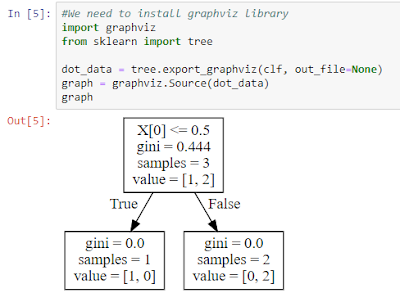
In the following example, we will try to fit a basic decision tree model to a three observations dataset.
#Simple example

from sklearn.tree import DecisionTreeClassifier
#X has 3 rows and two features
X = [[0, 0], [1, 1], [2,3]]

#Y has 3 rows
Y = [0, 1, 1]

#Instantiate decision tree
clf = DecisionTreeClassifier()

#Fit the decision tree to data
clf = clf.fit(X, Y)

# Predict class of new observation [0,0]
clf.predict([[0,0]])
Output: array([0]) Decision Tree prediction for the new observation [0,0] is class 0.
To know the prediction probabilities for the new observation:
>>> clf.predict_proba([[0., 0.]])
Output: array([[1., 0.]])
This gives prediction probabilities for the new observation [[0., 0.]].
In the output, first value of ‘1.’ indicates the probability that this observation belongs to class 0. The second value ‘0.’ gives the probability that the new observation belongs to class 1.
6. Default Hyperparameters of Decision Tree
The default hyperparameters of decision trees are given below:
DecisionTreeClassifier (class_weight=None, criterion=’gini’, max_depth=None, max_features=None, max_leaf_nodes=None, min_impurity_decrease=0.0, min_impurity_split=None, min_samples_leaf=1, min_samples_split=2, min_weight_fraction_leaf=0.0, presort=False, random_state=None, splitter=’best’)
These are the hyperparameters which we can change to improve the accuracy of the model. By default, gini function to measure the quality of the split in scikit-learn. To learn more about these, you may read scikit-learn manual.
7. Cross-validation
In another post, I will write about cross-validation in detail. For now, cross-validation is used to accurately measure the performance of any model, in this case, model is decision tree.
Data used is the famous Titanic dataset. For simplicity I have used only three features (sex, pclass and fare). And I have used 5-fold cross-validation (cv=5).
I have also divided the data into training (80%) and testing dataset (20%). I have calculated accuracy using both cv and also on test dataset.
from sklearn.model_selection import cross_val_score
from sklearn.tree import DecisionTreeClassifier
from sklearn.model_selection import train_test_split
from sklearn.metrics import accuracy_score

#Splitting
X_train, X_test, y_train, y_test = train_test_split(X, y, test_size=0.2, random_state=1)

#Instantiate decision tree model
DT = DecisionTreeClassifier(random_state=1)

#Fit decision tree
DT.fit(X_train, y_train)

#CV scores, 5 fold CV
scores = cross_val_score(DT, X_train, y_train, cv=5)

#Prediction and accuracy
y_pred = DT.predict(X_test)
accuracy_test = accuracy_score(y_test, y_pred)

#Print the summary
print("Accuracy: %0.2f (+/- %0.2f)" % (scores.mean(), scores.std() * 2))
print ("Test Accuracy: %0.2f" % (accuracy_test))
Accuracy: 0.79 (+/- 0.06) Test Accuracy: 0.82
8. Plotting Decision Trees
To plot decision trees, we need to install Graphviz.
For simplicity, I have used the same decision tree (clf) which we fitted earlier (in step 3) for plotting the tree.

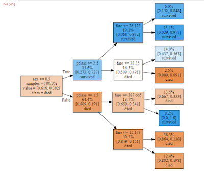
In the following example, I have used the decision tree model DT3 (where maximum depth was 3) for plotting the tree. We can rotate the tree, fill colours for easy understanding.
dot_data = tree.export_graphviz(DT3, out_file=None,
                         feature_names=['fare','sex','pclass'],
                         class_names=['died', 'survived'], #give it in ascending order (0 first, 1 later)
                                label = 'root', impurity =False, proportion =True,rotate =True, filled=True)
graph = graphviz.Source(dot_data)
graph

9. Tuning the decision tree
9.1 Manually tuning the hyperparameters
I have used five maximum depth values (3,4,5,6) for building the decision trees and to compare the accuracy.
from sklearn.model_selection import cross_val_score
from sklearn.tree import DecisionTreeClassifier
from sklearn.model_selection import train_test_split
from sklearn.metrics import accuracy_score

#Splitting
X_train, X_test, y_train, y_test = train_test_split(X, y, test_size=0.2, random_state=1)

#Instantiate
DTa = DecisionTreeClassifier(max_depth= None, random_state=1)
DTb = DecisionTreeClassifier(max_depth= 3, random_state=1)
DTc = DecisionTreeClassifier(max_depth= 4, random_state=1)
DTd = DecisionTreeClassifier(max_depth= 5, random_state=1)
DTe = DecisionTreeClassifier(max_depth= 6, random_state=1)

#Fit
DTa.fit(X_train, y_train)
DTb.fit(X_train, y_train)
DTc.fit(X_train, y_train)
DTd.fit(X_train, y_train)
DTe.fit(X_train, y_train)

#CV scores
scoresa = cross_val_score(DTa, X_train, y_train, cv=5)
scoresb = cross_val_score(DTb, X_train, y_train, cv=5)
scoresc = cross_val_score(DTc, X_train, y_train, cv=5)
scoresd = cross_val_score(DTd, X_train, y_train, cv=5)
scorese = cross_val_score(DTd, X_train, y_train, cv=5)

#Prediction and accuracy
y_preda = DTa.predict(X_test)
y_predb = DTb.predict(X_test)
y_predc = DTc.predict(X_test)
y_predd = DTd.predict(X_test)
y_prede = DTd.predict(X_test)

accuracy_testa = accuracy_score(y_test, y_preda)
accuracy_testb = accuracy_score(y_test, y_predb)
accuracy_testc = accuracy_score(y_test, y_predc)
accuracy_testd = accuracy_score(y_test, y_predd)
accuracy_teste = accuracy_score(y_test, y_prede)


#Print the summary
print("Accuracy unconstrained decision tree: %0.2f (+/- %0.2f)" % (scoresa.mean(), scoresa.std() * 2))
print ("Test Accuracy: %0.2f" % (accuracy_testa))

print("Accuracy (Max depth=3) : %0.2f (+/- %0.2f)" % (scoresb.mean(), scoresb.std() * 2))
print ("Test Accuracy: %0.2f" % (accuracy_testb))

print("Accuracy (Max depth=4) : %0.2f (+/- %0.2f)" % (scoresc.mean(), scoresc.std() * 2))
print ("Test Accuracy: %0.2f" % (accuracy_testc))

print("Accuracy (Max depth=5) : %0.2f (+/- %0.2f)" % (scoresd.mean(), scoresd.std() * 2))
print ("Test Accuracy: %0.2f" % (accuracy_testd))

print("Accuracy (Max depth=6) : %0.2f (+/- %0.2f)" % (scorese.mean(), scorese.std() * 2))
print ("Test Accuracy: %0.2f" % (accuracy_teste))
Accuracy unconstrained decision tree: 0.79 (+/- 0.06)
Test Accuracy: 0.82
Accuracy (Max depth=3) : 0.78 (+/- 0.05)
Test Accuracy: 0.85
Accuracy (Max depth=4) : 0.78 (+/- 0.05)
Test Accuracy: 0.82
Accuracy (Max depth=5) : 0.78 (+/- 0.04)
Test Accuracy: 0.83
Accuracy (Max depth=6) : 0.78 (+/- 0.04)
Test Accuracy: 0.83
9.2 Tuning the hyperparameters using GridSearchCV
Using GridSearchCV, we can find out the best possible combination of different hyperparameters which gives highest accuracy.
In the following example:
- I have used four maximum depth values (3,4,5,6) and two criteria (gini and entropy).
So there will be 4*2=8 possible combinations of hyperparameters.
#Let us run the same processing using GridSearch method

DT = DecisionTreeClassifier(random_state=1)

from sklearn.model_selection import GridSearchCV
params_DT = {'max_depth': [3, 4, 5, 6], 'criterion' : ["gini", "entropy"] }

Grid_DT = GridSearchCV(estimator=DT, param_grid=params_DT, cv=5)

Grid_DT.fit(X_train, y_train)
GridSearchCV gives the best combination of hyperparameters which gives highest accuracy among the possible combinations.
In [55]: print(‘Best hyerparameters:’, Grid_DT.best_params_)
Out[55]: Best hyerparameters: {‘criterion’: ‘gini’, ‘max_depth’: 6}
The accuracy score of the best model is given below:
In [56]: Grid_DT.best_score_
Out[56]: 0.7829827915869981.
Summary
In this post, we have explored:
- What are decision trees
- When to use decision trees
- Advantages
- Disadvantages and possible steps to overcome
- Examples
- Cross-validation
- Visualizing decision trees
- GridSearchCV for hyperparameter tuning in decision trees
If you have any questions or suggestions, please do share. I will be happy to interact.

