Logistic regression is a supervised learning technique applied to classification problems.
In this post, let us explore:
- Logistic Regression model
- Advantages
- Disadvantages
- Example
- Hyperparemeters and Tuning
Logistic Regression model
Logistic functions capture the exponential growth when resources are limited.
Sigmoid function is a special case of Logistic function as shown in the picture below (link). In the following pictures, I have shown how to derive the log of odds ratio from the sigmoid function.

Use sigmoid function to model the probability of dependent variable being 1 or 0 (binary classification).

Now we will see how to derive the log of odds ratio [p/(1-p)].

As shown in the pictures above, log of odds ratio (logit) is linear function of independent variables.
Advantage
- We can interpret the coefficients (white box model)
We can interpret the results based on the size and sign of the regression coefficients. This is useful to identify the relationship between independent and dependent variables.
Disadvantage
- Requires that each data point be independent of other data points (source)
Example
The data used for demonstrating the logistic regression is from the Titanic dataset. For simplicity I have used only three features (Age, fare and pclass).
And I have performed 5-fold cross-validation (cv=5) after dividing the data into training (80%) and testing (20%) datasets. I have calculated accuracy using both cv and also on test dataset.
#Ravel
y=y.values.ravel()

from sklearn.linear_model import LogisticRegression
from sklearn.model_selection import train_test_split

#Splitting
x_train, x_test, y_train, y_test = train_test_split(X, y, test_size=0.2, random_state=0)

#LR model
logisticRegr = LogisticRegression()

#Fit
logisticRegr.fit(x_train, y_train)
LogisticRegression(C=1.0, class_weight=None, dual=False, fit_intercept=True, intercept_scaling=1, max_iter=100, multi_class=’ovr’, n_jobs=1, penalty=’l2′, random_state=None, solver=’liblinear’, tol=0.0001, verbose=0, warm_start=False)
The above output shows the default hyperparemeters used in sklearn.
Let us now perform the 5-fold cross-validation and find out the accuracy.
from sklearn.model_selection import cross_val_score
from sklearn.metrics import accuracy_score

#CV scores, 5 fold CV
scores = cross_val_score(logisticRegr, x_train, y_train, cv=5)

#Prediction and accuracy
y_pred = logisticRegr.predict(x_test)
accuracy_test = accuracy_score(y_test, y_pred)

#Print the summary
print("Accuracy: %0.2f (+/- %0.2f)" % (scores.mean(), scores.std() * 2))
print ("Test Accuracy: %0.2f" % (accuracy_test))
Accuracy: 0.68 (+/- 0.04)
Test Accuracy: 0.70
# Score
score = logisticRegr.score(x_test, y_test)
print ("Accuracy: %0.2f" % (score))

#Prediction
predictions = logisticRegr.predict(x_test)
predictions
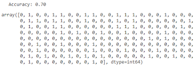
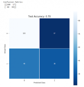
To get the confusion matrix, we can use the following code. We can also visualize the confusion matrix for easier understanding.
from sklearn import metrics
import matplotlib.pyplot as plt
import seaborn as sns
from sklearn import metrics

#confusion matrix
cm = metrics.confusion_matrix(y_test, predictions)
print("Confusion Matrix: \n", cm)

#Visualize the confusion matrix
plt.figure(figsize=(9,9))
sns.heatmap(cm, annot=True, fmt=".0f", linewidths=.5, square = True, cmap = 'Blues_r');
plt.ylabel('Actual Class');
plt.xlabel('Predicted Class');
all_sample_title = "Test Accuracy: %0.2f" % (score)
plt.title(all_sample_title, size = 15);
Hyperparameters
Let us look at the important hyperparameters of Logistic Regression one by one in the order of sklearn’s fit output. The following output shows the default hyperparemeters used in sklearn.
    LogisticRegression(C=1.0, class_weight=None, dual=False, fit_intercept=True,
          intercept_scaling=1, max_iter=100, multi_class='ovr', n_jobs=1,
          penalty='l2', random_state=None, solver='liblinear', tol=0.0001,
          verbose=0, warm_start=False)
- C
- It is the inverse of regularization strength. Lower the value of C, higher the regularization and hence lower is the chance of overfitting. Default is C=1.
- Class weight
- By default, sklearn uses ‘balanced’ mode by automatically adjusting the class weights to inverse of frequencies in each class. This is useful while handling class imbalance in dataset.
- Fit Intercept
- By default, intercept is added to the logistic regression model.
- Multiclass
- In this we have three options: ovr’, ‘multinomial’, ‘auto’. ‘ovr’ corresponds to One-vs-Rest. Auto selects ‘ovr’ when problem is binary classification, otherwise ‘multinomial’. These are commonly tuned hyperparameters. For more about these read sklearn’s manual.
Tuning the Hyperparameters
Now let us tune the hyperparameters using GridSearch.
#import GridseachCV
from sklearn.model_selection import GridSearchCV

#Instantiate
clf = LogisticRegression()

#Grid
parameter_grid = {'C': [0.01, 0.1, 1, 2, 10, 100], 'penalty': ['l1', 'l2']}

#Gridsearch
gridsearch = GridSearchCV(clf, parameter_grid)
gridsearch.fit(x_train, y_train);

#Get best hyperparameters
gridsearch.best_params_
{‘C’: 2, ‘penalty’: ‘l2’}
Then you can use these values in the pipeline for fitting the model.
We can also use randomized search for finding the best parameters. Advantages of randomized search is that it is faster and also we can search the hyperparameters such as C over distribution of values.
References
https://scikit-learn.org/stable/modules/generated/sklearn.linear_model.LogisticRegression.html

